GPU Profiling for LLM Fine-Tuning on DGX Spark: What the Traces Reveal
I fine-tuned a 1.5B parameter model on a DGX Spark and the training finished in 26 seconds. Good enough? I had no idea. The terminal showed 2.18 it/s and a loss curve that went down. But whether the GPU was actually working hard or mostly waiting around — that, the training logs don’t tell you.
So I profiled it. What I found was that a machine with 130 GB of unified GPU memory was spending 74% of its CUDA API time on memory copies, and GPU utilization dropped as low as 18.6% during warmup. For a quick LoRA run on a small model, this doesn’t matter. For scaling to production workloads, it’s exactly the kind of thing that turns a 2-hour job into an 8-hour one.
This post walks through what GPU profiling actually reveals about LLM fine-tuning, how to read the traces, and what to do about the bottlenecks.
The Setup
The workload is straightforward: LoRA fine-tuning of Qwen2.5-1.5B-Instruct on 200 samples from the Databricks Dolly-15k dataset. Deliberately small — the goal is profiling, not training a production model.
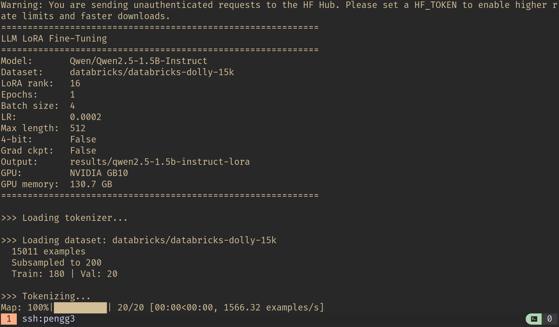 Training configuration: Qwen2.5-1.5B-Instruct on the NVIDIA GB10 with 130.7 GB unified memory.
| Parameter | Value |
|---|---|
| Model | Qwen/Qwen2.5-1.5B-Instruct |
| Method | LoRA (rank 16, alpha 32) |
| Trainable params | 18.5M / 1.6B total (1.18%) |
| Dataset | databricks-dolly-15k (200 samples: 180 train / 20 val) |
| Epochs | 1 |
| Batch size | 4 |
| Max sequence length | 512 |
| Learning rate | 2e-4 (cosine schedule) |
| Precision | bf16 |
| GPU | NVIDIA GB10 (DGX Spark) |
| GPU memory | 130.7 GB unified |
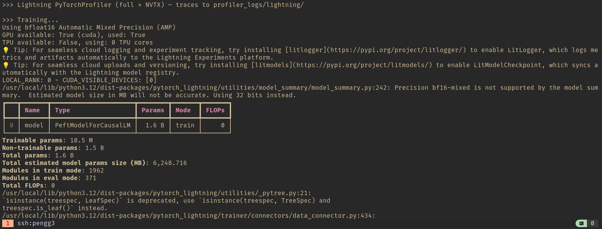 Model summary: 18.5M trainable parameters out of 1.6B total. The LoRA adapters are a thin layer on top of frozen weights.
Training completed in 26 seconds — 12 steps at 2.18 iterations per second in steady state:
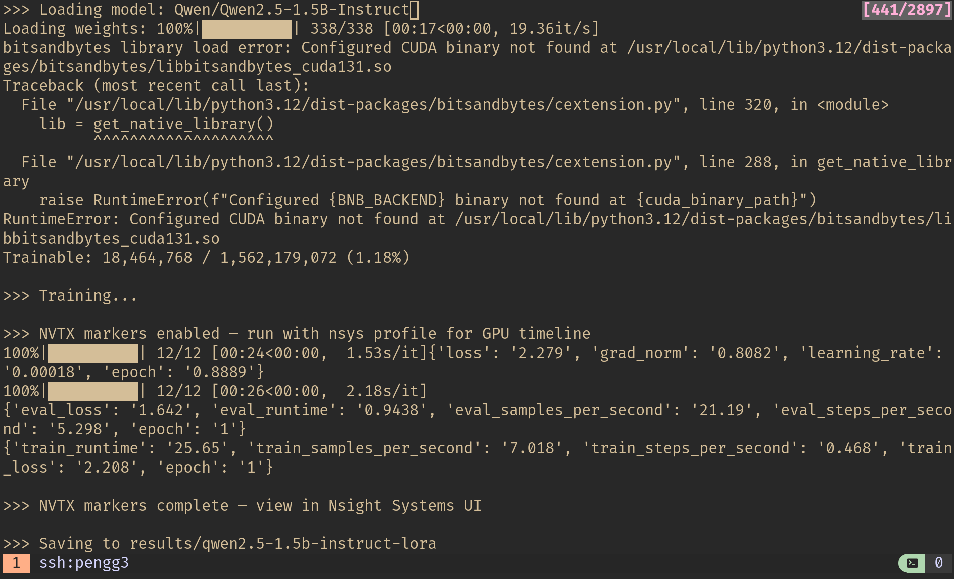 Terminal output: 12 training steps, train_runtime 25.65s, eval_loss 1.642. The first few iterations run at 1.53s/it during warmup before settling to 2.18 it/s.
Two Profilers, Two Perspectives
I instrumented the training run with two profiling tools to see what each one captures:
torch.profiler — PyTorch’s built-in profiler. Captures operator-level timing (which aten:: ops are running), CUDA kernel durations, and memory allocation. Produces a Chrome-compatible trace JSON you can open in chrome://tracing or Perfetto UI. Best for understanding what PyTorch is doing.
NVIDIA Nsight Systems — a system-level profiler that captures everything: CUDA API calls, GPU kernel execution, memory transfers, CPU thread activity, OS runtime calls. This is the one that shows you the full picture — not just what’s running, but what’s waiting.
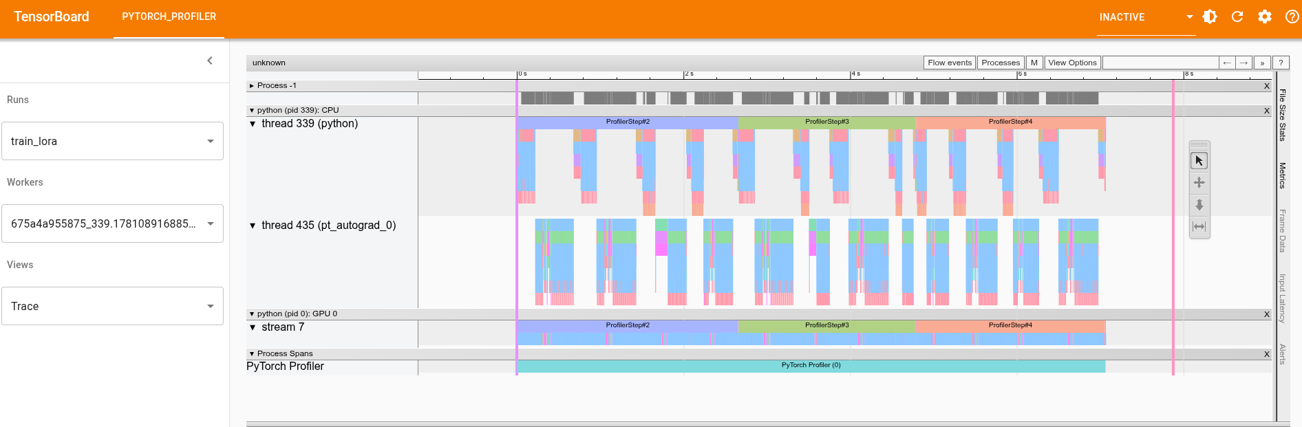
Here’s the TensorBoard trace view from torch.profiler, showing the same training run from a different angle:
 TensorBoard’s Trace view: CPU thread (top) shows operator execution,
 pt_autograd_0 shows backward pass activity, and GPU stream 7 shows the actual kernel execution. The ProfilerStep#2, #3, #4 markers delineate individual training steps.
The torch.profiler trace is useful for zooming into individual operators and their call stacks. But for system-level insights — where the GPU is idle and why — Nsight Systems is where the interesting findings are.
Reading the Nsight Systems Timeline
Opening the .nsys-rep file in nsys-ui gives you a timeline view of the entire 56-second trace.
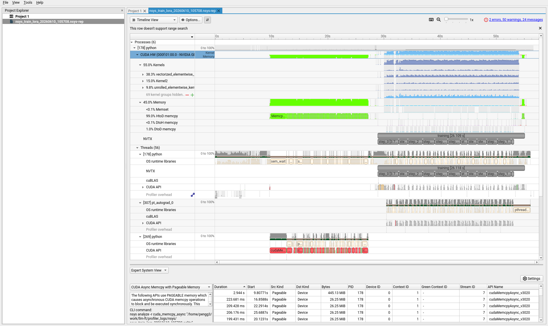 The Nsight Systems timeline. Top rows: GPU hardware activity (kernels in green, memory in pink). Middle: NVTX markers showing the
 training [26.118 s] region with individual step markers. Bottom: thread-level CPU activity.
The trace breaks into two clear phases:
- 0–28 seconds: Model loading, tokenization, CUDA context initialization. Sparse GPU activity — mostly memory copies loading the 1.6B parameter model onto the device.
- 28–56 seconds: The actual training loop. Dense GPU activity with 12 training steps visible in the NVTX row.
The rows that matter most:
| Row | What it shows |
|---|---|
| CUDA HW → Kernel | Actual GPU compute. Green blocks = the GPU is working. Gaps = the GPU is idle. |
| CUDA HW → Memory | Device memory transfers. Pink blocks = data movement. |
| NVTX | Named regions from the training code — training, step_0, step_2, etc. |
| cuBLAS | Matrix multiplication calls — the core of transformer compute. |
| CUDA API | Host-side CUDA calls. Long bars here mean the CPU is blocking. |
Scrolling down reveals the thread-level view:
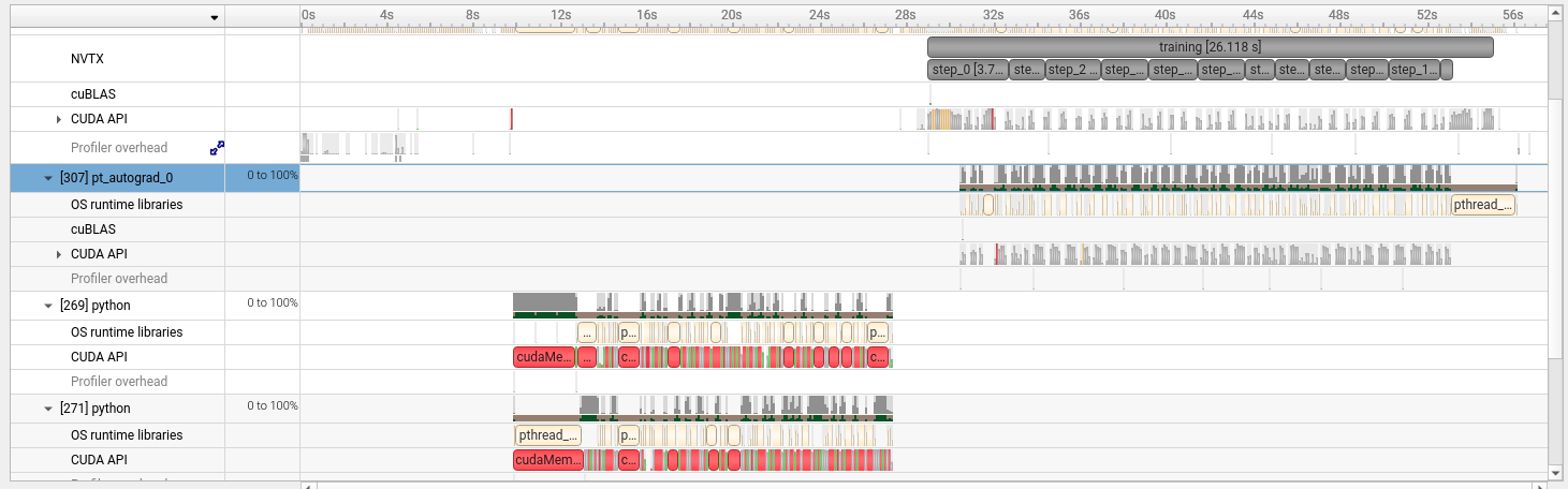 The
The pt_autograd-0 thread activates during the training region (backward pass). Below it, data loader threads show cudaMemcpy and pthread activity during model loading.
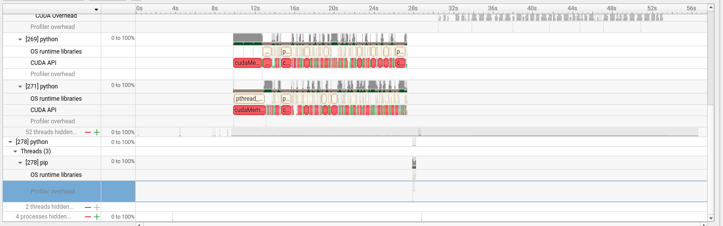 Multiple Python processes handle data loading. The red and green blocks in the CUDA API rows are
 cudaMemcpy and cudaMalloc calls during the setup phase.
Finding 1: GPU Utilization Has Two Soft Spots
The Expert System View at the bottom of Nsight Systems runs automated analysis rules against the trace. The GPU Utilization rule flagged two time regions where utilization dropped below 50%:
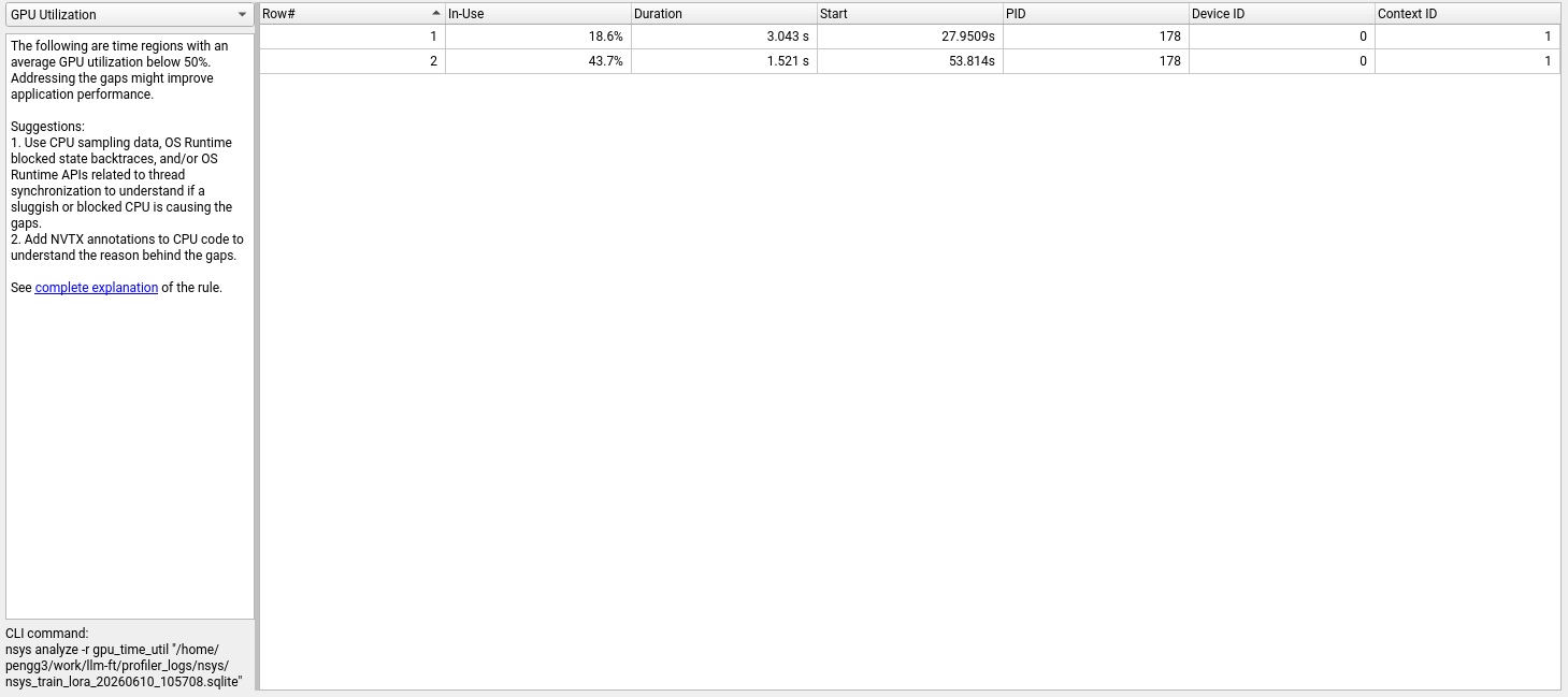 Two underutilized regions: 18.6% for 3.04 seconds at the start of training, and 43.7% for 1.52 seconds near the end.
| Region | GPU Utilization | Duration | When |
|---|---|---|---|
| 1 | 18.6% | 3.04 s | 27.95 s (training start) |
| 2 | 43.7% | 1.52 s | 53.81 s (near training end) |
The first region (18.6%) aligns with the beginning of the training loop — CUDA JIT compilation, cuBLAS handle creation, and the first forward pass through the model. The GPU is mostly waiting for the runtime to warm up.
The second region (43.7%) corresponds to the final step and evaluation pass, where the workload is smaller and there’s cleanup overhead.
Finding 2: Two GPU Gaps Longer Than 500ms
The GPU Gaps rule identifies stretches where the GPU had no work at all:
 Two idle gaps: 854ms and 561ms, both at the transition from model loading to training.
Both gaps occur right around the 28–30 second mark — the transition from model setup to the training loop. The GPU finishes loading weights, then waits 854ms before the first training kernel launches. This is the CUDA warmup penalty: the first kernel compilation, memory pool initialization, and cuBLAS workspace allocation all happen here.
For a 26-second training run, 1.4 seconds of GPU idle time is 5.4% of the total. For a multi-hour production run, this fixed cost amortizes away. But it’s a reminder that short profiling runs overweight startup costs.
Finding 3: 74% of CUDA API Time Is Memory Copies
This is the most striking finding. The CUDA API summary from nsys stats reveals where the host-side time goes:
| API Call | Time (%) | Total Time | Calls |
|---|---|---|---|
cudaMemcpyAsync | 74.2% | 65.7 s | 6,292 |
cudaLaunchKernel | 12.7% | 11.2 s | 273,186 |
cudaMalloc | 4.6% | 4.06 s | 436 |
cudaStreamSynchronize | 2.7% | 2.35 s | 3,380 |
Memory copies dominate. The Expert System flags this specifically as CUDA Async Memcpy with Pageable Memory:
 The pageable memory warning. Each row is a
 cudaMemcpyAsync call that was forced to run synchronously because the host memory wasn’t pinned.
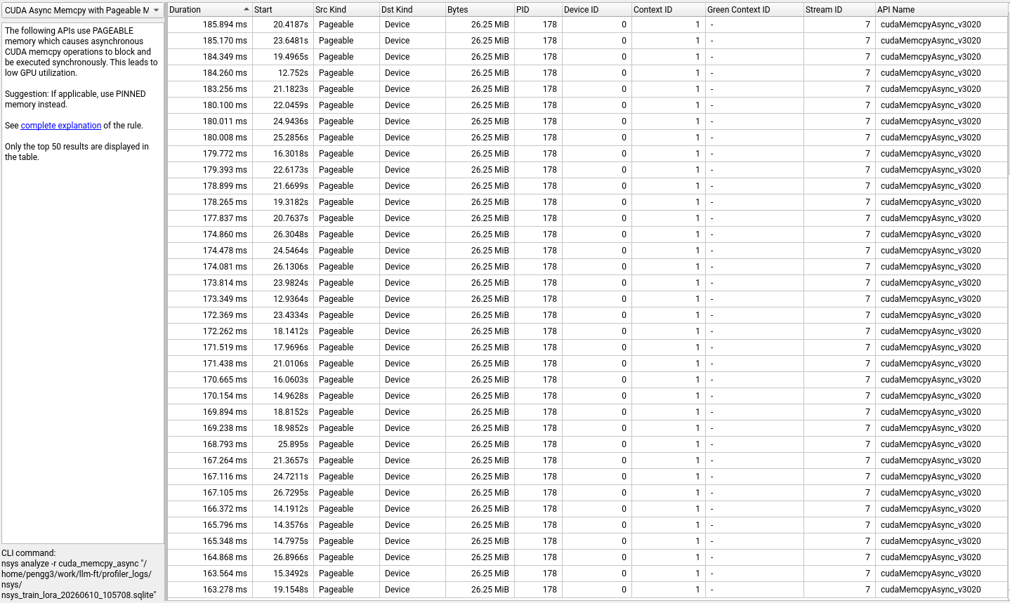 The transfers: dozens of 26.25 MiB chunks taking 170–224ms each, plus one 445.13 MiB transfer that took 2.94 seconds.
The issue: when CUDA copies data from host to device using pageable (regular) memory, it can’t use DMA directly. Instead, it first copies to a pinned staging buffer, then transfers to the GPU. This makes cudaMemcpyAsync effectively synchronous — the “async” in the name becomes a lie.
This is overwhelmingly a model loading cost, not a per-step training cost. The 1.6B parameter model is loaded from disk into pageable CPU memory by HuggingFace transformers, then copied chunk by chunk to the GPU. Each 26.25 MiB chunk corresponds to a model layer’s weight tensor.
A caveat for this hardware: The DGX Spark uses unified memory where CPU and GPU share the same physical memory pool. On this architecture, “copies” may be logical page migrations rather than physical data transfers across a bus. The 74% figure reflects the software overhead of the pageable memory path, but the actual wall-clock impact may be smaller than on a discrete GPU with separate device memory. More on this in the Diagnostics section below.
Finding 4: Synchronization APIs Add Friction
The CUDA Synchronous APIs view shows every call that forces the CPU to wait for the GPU:
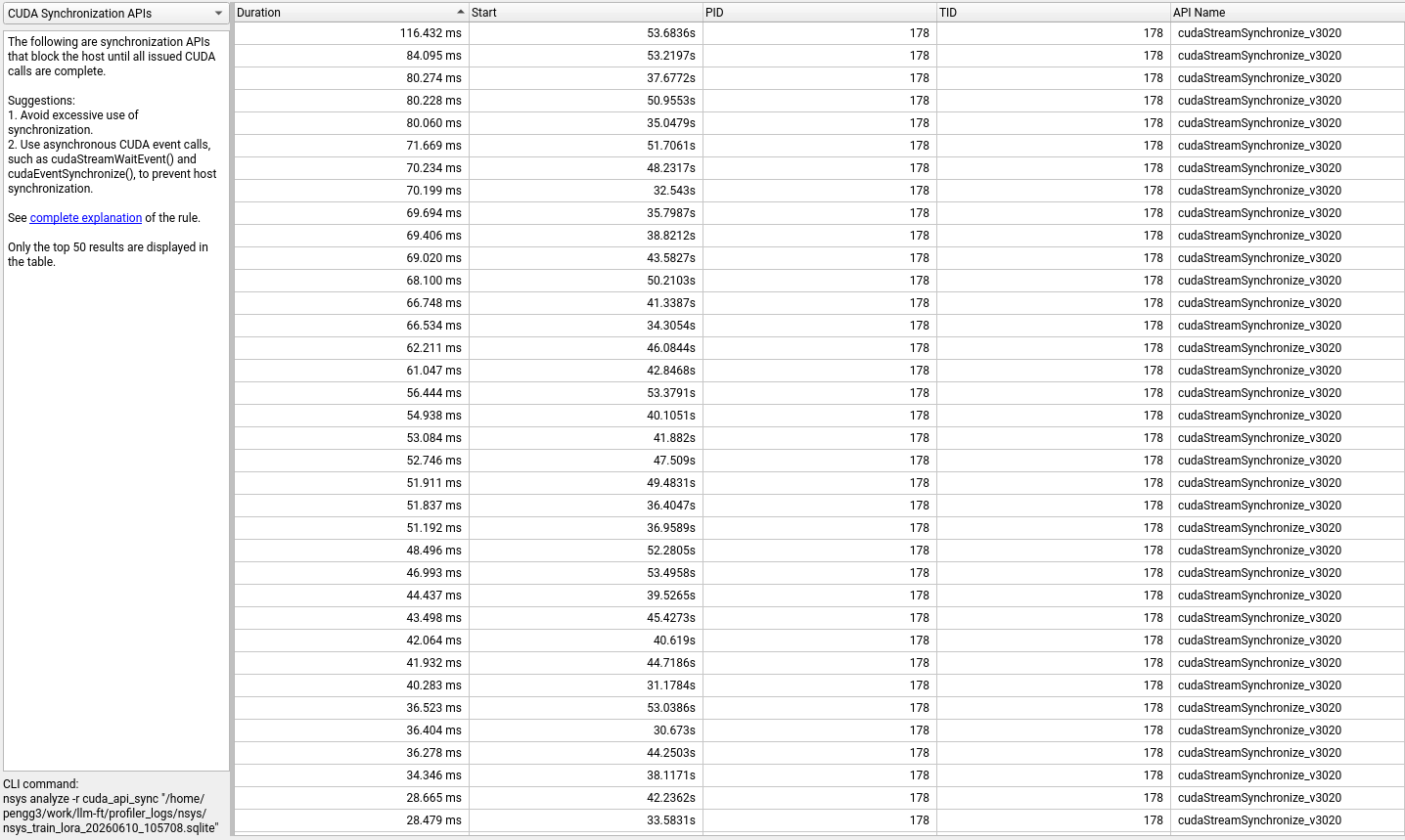 Synchronization calls, sorted by duration. Each
 cudaStreamSynchronize stalls the CPU until all GPU work on that stream completes.
The 3,380 cudaStreamSynchronize calls total 2.35 seconds. Most are short (the median is sub-millisecond), but the long tail includes calls exceeding 100ms. These are points where the CPU-GPU pipeline stalls — the CPU can’t queue new work until the GPU catches up. In a well-pipelined training loop, you’d want near-zero synchronization during steady-state steps.
Finding 5: Step Times Vary Wildly
The NVTX summary reveals that not all training steps are created equal:
| Step | Duration |
|---|---|
| step_0 | 3.74 s |
| step_2 | 2.63 s |
| step_10 | 2.39 s |
| step_4 | 2.27 s |
| step_5 | 2.24 s |
| step_3 | 2.11 s |
| step_9 | 1.97 s |
| step_8 | 1.70 s |
| step_1 | 1.66 s |
| step_7 | 1.56 s |
| step_6 | 1.37 s |
| step_11 | 0.40 s |
Step_0 takes 3.74 seconds — nearly 10x longer than step_11 at 0.40 seconds. The first step includes CUDA kernel JIT compilation and memory pool warmup, so a 2–3x overhead is expected. But the variance across mid-training steps (1.37s to 2.63s) suggests something else: variable sequence lengths in the input batches.
With max_length=512 and no sequence packing, each batch pads to the longest sequence in that batch. A batch where the longest sample is 500 tokens costs more than one where it’s 200 tokens, because every attention and feedforward operation scales with sequence length. The Dolly-15k dataset has widely varying instruction lengths, which explains the step-to-step variance.
Finding 6: Where the GPU Cycles Actually Go
The top GPU kernels by time tell you what the hardware is spending its cycles on:
| Kernel | Time (%) | Instances | What it does |
|---|---|---|---|
unrolled_elementwise_kernel (copy) | 9.8% | 42,037 | Tensor copies and type conversions |
vectorized_elementwise_kernel (add) | 8.2% | 31,230 | Element-wise additions |
bfloat16_copy_kernel | 7.3% | 43,600 | bf16 precision format conversions |
| CUTLASS GEMM (tn) | 5.9% | 9,296 | Matrix multiplications (linear layers) |
vectorized_elementwise_kernel (mul) | 5.3% | 3,920 | Element-wise multiplications |
| Softmax forward | 3.3% | 50 | Attention softmax |
nvjet GEMM variants | ~12% | various | Optimized matrix multiplies |
| Memory-efficient attention backward | 2.4% | 896 | Attention gradient computation |
The torch.profiler view confirms this pattern from the operator level:
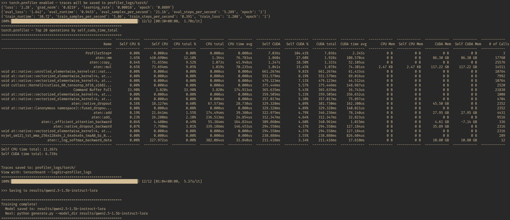 torch.profiler’s top 20 operations sorted by self CUDA time.
 aten::mm (matrix multiply) takes 27.6% of CUDA time with 17,760 calls allocating 86.3 GB. aten::copy_ at 18.5% reflects the data movement overhead. aten::mul at 15.5% covers element-wise operations across 14,511 calls. Self CUDA time totals 6.74s across 3 profiled steps.
The takeaway: the GPU is spending roughly 17% of its kernel time on data movement (copies, format conversions) and 24% on GEMM and attention compute. The remaining time is spread across element-wise operations (activations, normalization, gradient scaling) and many smaller kernels not shown in this table.
This ratio is typical for a 1.5B model. Larger models shift the balance toward compute because GEMM operations scale quadratically with hidden dimension (both input and output dimensions grow together), while element-wise operations scale linearly.
Diagnostics: The Unified Memory Note
The diagnostics panel flagged an interesting message:
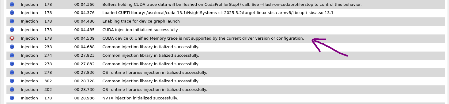 “CUDA device 0: Unified Memory trace is not supported by the current driver version or configuration.”
The DGX Spark’s GB10 uses unified memory — CPU and GPU share the same physical memory pool, which is fundamentally different from discrete GPU architectures where data must be explicitly copied across PCIe. This means some of the cudaMemcpyAsync overhead we measured may be overstated: in unified memory, “copies” can be logical rather than physical, depending on the memory access pattern and page migration policy.
This is a profiling limitation to be aware of. The pageable memory warnings are still valid (the software path is suboptimal), but the actual performance impact on unified memory hardware may be smaller than the numbers suggest.
What This Means for Scaling Up
The profiling data points to a clear optimization path for taking this workload from a 200-sample experiment to production scale:
Short-term: Fix the Easy Wins
1. Use pinned memory for data loading. Finding 3 showed that 74% of CUDA API time went to cudaMemcpyAsync, with Nsight Systems flagging pageable memory as the cause. Setting pin_memory=True in the DataLoader and dataloader_pin_memory=True in TrainingArguments tells PyTorch to load data into a special area of CPU memory that the GPU can read from directly, skipping the extra internal copy that the pageable memory warning describes. That said, we didn’t profile with vs. without pinned memory, so we can’t say exactly how much it would help here. In general practice, the speedup per batch is usually small — maybe a millisecond or two — because data transfer is rarely the bottleneck during training. It’s still worth turning on as a reasonable default since it costs almost nothing. On unified memory architectures like the GB10, the benefit may be even smaller since CPU and GPU share the same physical memory. The things that matter more for data loading speed are using enough num_workers and making sure data preparation overlaps with training.
2. Use CUDA graphs or torch.compile. Every time PyTorch runs an operation (a matrix multiply, an addition, a ReLU), it makes a separate call to the GPU to launch it. Each call has a small overhead, but the trace shows 273,186 of them, adding up to 12.7% of total API time just on the overhead of asking the GPU to do work. torch.compile addresses this by analyzing the computation graph and fusing multiple small operations into fewer, larger GPU kernels — so instead of launching many separate kernels, it generates one that does several steps at once. CUDA graphs take a different approach: they record a sequence of GPU operations once, then replay the entire sequence with a single CPU call, nearly eliminating launch overhead for repeated computations like training steps.
3. Adopt sequence packing. Finding 5 showed step times ranging from 0.40s to 3.74s, which we attributed to variable sequence lengths in the Dolly dataset. The profiler showed the symptom — sequence packing is a common solution, though not something the trace directly prescribed. When sequences in a batch have different lengths, the short ones get padded to match the longest one. The GPU does the same amount of work on padding tokens as on real tokens — that’s wasted compute. Sequence packing solves this by concatenating multiple shorter sequences into a single max_length slot, so the GPU spends less time on empty padding. This matters most when your data has widely varying lengths. For example, protein language models often deal with sequences ranging from a few dozen amino acids to thousands — without packing, a batch with one long protein wastes enormous compute on padding the short ones. That said, part of that variance is real — longer sequences legitimately take more compute. Packing makes step times more consistent, but the total compute across a full epoch may not drop dramatically. The win is more about predictable throughput and better GPU utilization than a big speedup. Libraries like flash-attn and HuggingFace’s DataCollatorWithFlattening support packing.
Medium-term: Scale the Workload
4. Increase batch size. The profiling showed 273,186 kernel launches (12.7% of API time) and 3,380 synchronization calls (2.35 seconds) across 12 training steps. These per-step overheads are fixed costs — they happen regardless of how much data is in each batch. Increasing batch size would spread these costs across more data per step, which could improve GPU utilization during steady-state training. We didn’t measure peak memory usage in this profiling run, so it’s hard to say exactly how much headroom is available, but a 1.6B model on 130.7 GB of unified memory likely leaves room to experiment with larger batches.
5. Profile with larger models. The kernel breakdown in Finding 6 showed roughly 17% of GPU time on data movement (copies, format conversions) and 24% on GEMM compute. In a small model like 1.5B, the weight matrices are relatively small, so the matrix multiplications (the core math in attention and feedforward layers) finish quickly, and the GPU ends up spending a comparable amount of time on housekeeping — copying data, converting formats, moving things around. In a larger model, each matrix multiplication does much more work per call, but the housekeeping doesn’t grow nearly as fast. So the balance would likely shift toward compute taking a larger share of GPU time. A profiling run with a 7B+ model would reveal whether the bottlenecks look different at production scale.
Production: Sustained Training
6. Profile steady-state only. As we saw in Findings 2 and 5, the first few steps are dominated by startup costs — CUDA warmup, kernel compilation, memory pool initialization. Step_0 took 3.74 seconds while later steps settled around 1.5–2 seconds. In a 12-step run, these startup costs make up a large share of the total time and can skew the picture. For production profiling, you’d want to skip the warmup phase entirely and capture only the steady-state training window. Nsight Systems supports this with --delay and --duration flags, letting you start recording after the first few steps have already completed.
The Bigger Picture
GPU profiling isn’t something most ML engineers do regularly. We run training, check the loss curve, and move on. But the traces tell a story that loss curves can’t: a 1.5B model on a 130 GB unified-memory GPU is compute-limited in the kernels and bandwidth-limited in between. The GPU alternates between bursts of matrix multiplication and stretches of copying data, converting formats, and waiting for synchronization.
For small experiments, none of this matters — 26 seconds is 26 seconds. But the patterns revealed at small scale predict the bottlenecks at large scale. The model-loading overhead is a fixed cost that amortizes over longer runs, but the per-step inefficiencies don’t: step time variance from uneven sequence lengths, synchronization stalls between CPU and GPU, suboptimal kernel launch patterns. These compound over thousands of steps.
Twenty-six seconds felt fast until I opened the trace and saw how much of it was wasted. The profiler won’t make your training faster — but without it, you’re guessing which knobs to turn.