Beta Distribution: Part 3 - Connection to Order Statistics

Order statistics play a crucial role in probability and statistics, particularly in quantile estimation, reliability analysis, and extreme value theory. In previous posts, we’ve explored the Beta distribution from Bayesian and frequentist perspectives. Now, let’s uncover another insightful connection: the relationship between order statistics and the Beta distribution.

We’ll begin by defining order statistics, carefully derive their cumulative distribution function (CDF) using indicator variables and Bernoulli trials, demonstrate their probability density function (PDF) with a detailed multinomial framework, and ultimately highlight their elegant connection to the Beta distribution when sampling from a Uniform(0,1) distribution.

What Are Order Statistics?

Given a random sample of size \(n\):

\[X_1, X_2, \dots, X_n\]

We sort these values in ascending order:

\[X_{(1)} \leq X_{(2)} \leq \dots \leq X_{(n)}\]

Here:

• \(X_{(1)}\) is the minimum.
• \(X_{(k)}\) is the \(k\)-th smallest value.
• \(X_{(n)}\) is the maximum.

These sorted values, \(X_{(k)}\), are called k-th order statistics.

Deriving the CDF of the \(k\)-th Order Statistic

The cumulative distribution function (CDF) of the \(k\)-th order statistic \(X_{(k)}\) is defined as:

\[F_{X_{(k)}}(x) = P(X_{(k)} \leq x)\]

This represents the probability that at least \(k\) of the \(n\) sample values are less than or equal to \(x\).

Step 1: Defining Indicator Variables

Define an indicator variable \(I_i\) for each sample value \(X_i\):

\[I_i = \begin{cases} 1, & \text{if } X_i \leq x \\[6pt] 0, & \text{if } X_i > x \end{cases}\]

Each \(I_i\) is a Bernoulli random variable with probability of success \(F_X(x)\):

\[I_i \sim \text{Bernoulli}(F_X(x)), \quad \text{since} \quad P(X_i \leq x) = F_X(x)\]

because the original sample \(X_1, X_2, \dots, X_n\) is i.i.d.

Step 2: Counting the Number of Values ≤ \(x\)

Define the random variable \(S\) to count how many of the \(n\) values are less than or equal to \(x\):

\[S = \sum_{i=1}^{n} I_i\]

Since \(S\) is the sum of \(n\) independent Bernoulli random variables, it follows a Binomial distribution:

\[S \sim \text{Binomial}(n, F_X(x))\]

Step 3: Computing \(P(X_{(k)} \leq x)\)

To have \(X_{(k)} \leq x\), at least \(k\) of the \(n\) values must be ≤ \(x\). Therefore, this is equivalent to having \(S \geq k\), where \(S \sim \text{Binomial}(n, F_X(x))\):

\[\begin{aligned} P(X_{(k)} \leq x) &= P(S \geq k) \\ &= 1 - P(S \leq k - 1) \\ &= 1 - \sum_{j=0}^{k-1} \binom{n}{j} [F_X(x)]^j [1 - F_X(x)]^{n - j} \\ &= \sum_{j=k}^{n} \binom{n}{j} [F_X(x)]^j [1 - F_X(x)]^{n - j} \end{aligned}\]

Thus, the simplified final form of the CDF for the \(k\)-th order statistic is explicitly represented as the sum of binomial probabilities from \(j = k\) to \(j = n\):

\[\boxed{F_{X_{(k)}}(x) = \sum_{j=k}^{n} \binom{n}{j}[F_X(x)]^j[1 - F_X(x)]^{n - j}}\]

Deriving the PDF of the \(k\)-th Order Statistic

For \(X_{(k)}\) to be in a small interval \([x, x+dx)\), the sample must satisfy:

• Exactly \(k-1\) observations are less than \(x\),
• Exactly one observation lies in \([x, x+dx)\),
• Exactly \(n - k\) observations are greater than \(x+dx\).

The number of ways to assign \(n\) observations to these groups is given by the multinomial coefficient:

\[\frac{n!}{(k-1)! \cdot 1! \cdot (n-k)!}\]

The probability of one specific assignment is:

\[[F_X(x)]^{k-1}[f_X(x)dx][1 - F_X(x)]^{n-k}\]

Multiplying, the total probability is:

\[P(x \leq X_{(k)} < x+dx) = \frac{n!}{(k-1)!(n-k)!}[F_X(x)]^{k-1}[1 - F_X(x)]^{n-k}f_X(x)dx\]

Dividing by \(dx\) gives the PDF:

\[\boxed{f_{X_{(k)}}(x) = \frac{n!}{(k-1)!(n-k)!}[F_X(x)]^{k-1}[1 - F_X(x)]^{n-k}f_X(x)}\]

Connection to the Beta Distribution

An elegant connection arises when the original observations are from \(\text{Uniform}(0,1)\) distribution. Specifically, if \(X_i \sim \text{Uniform}(0,1)\):

• CDF: \(F_X(x) = x\) for \(0 < x < 1\).
• PDF: \(f_X(x) = 1\) for \(0 < x < 1\).

Substituting these into our order statistic PDF formula gives:

\[f_{X_{(k)}}(x) = \frac{n!}{(k-1)!(n-k)!} x^{k-1}(1 - x)^{n-k}, \quad 0 < x < 1\]

Now, let’s recall the PDF of the Beta distribution with parameters \(\alpha\) and \(\beta\):

\[f(x; \alpha, \beta) = \frac{x^{\alpha-1}(1-x)^{\beta-1}}{B(\alpha,\beta)}, \quad 0 < x < 1\]

where the Beta function \(B(\alpha,\beta)\) for integer arguments is:

\[B(\alpha,\beta) = \frac{(\alpha-1)!(\beta-1)!}{(\alpha+\beta-1)!}\]

Set \(\alpha = k\) and \(\beta = n - k + 1\). Then we have:

\[f(x; k, n - k + 1) = \frac{x^{k-1}(1 - x)^{n - k}}{B(k, n - k + 1)} = \frac{n!}{(k-1)!(n-k)!} x^{k-1}(1 - x)^{n-k}\]

Notice this matches exactly our derived order statistic PDF. Hence, we confirm the beautiful relationship explicitly:

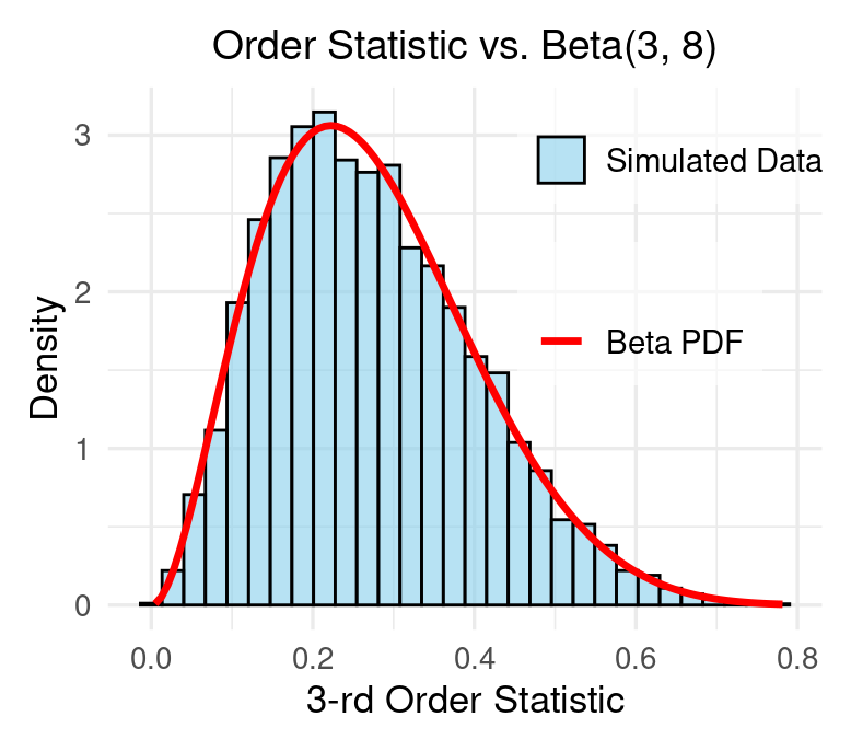
\[X_{(k)} \sim \text{Beta}(k, n - k + 1), \quad X_i \sim \text{Uniform}(0,1)\]

Visualization via R Simulation

Here’s an R simulation illustrating this relationship:

library(ggplot2)

n <- 10; k <- 3; sims <- 10000
set.seed(123)

# Simulate k-th order statistic
order_stats <- replicate(num_sim, sort(runif(n))[k])

ggplot(data.frame(Value = order_stats), aes(x = Value)) +
  geom_histogram(aes(y = ..density..)) +
  stat_function(fun = dbeta, args = list(shape1 = k, shape2 = n - k + 1), color = 'red') +
  labs(title = "Order Statistic vs. Beta(3,8)") +
  theme_minimal()

Conclusion

In this post, we rigorously derived the CDF and PDF of order statistics, revealing their profound connection to the Beta distribution for uniformly sampled data. These insights highlight the elegant structures underlying statistics.