Beta Distribution: Part 2.1 - Frequentist Perspectives - Clopper–Pearson Intervals

Beta Distribution in Frequentist Inference

In my previous post, I explored the basic properties of the Beta distribution and its role in Bayesian statistics. In this post, I shift focus to the frequentist perspective, examining how the Beta distribution appears in classical statistical methods like confidence interval construction, hypothesis testing and estimations.

This installment (Part 2.1) focuses on the Clopper–Pearson confidence intervals for proportions, a method that directly leverages the Beta distribution to ensure exact coverage. Beyond this specific application, my aim is to build a deeper intuition for the Beta distribution, enabling connections between different statistical concepts and better understanding the principles underpinning these methods.

Confidence Intervals for Proportions (Clopper–Pearson)

When observing a binomial outcome, such as \(k\) successes out of \(n\) trials, the most straightforward estimate of the probability of success \(p\) is the sample proportion \(\hat{p} = k / n\). Constructing a confidence interval for \(p\) can be done using various methods, including the Wald interval, Wilson interval, and others. Among these, the Clopper–Pearson interval is a classic “exact” method that directly incorporates the Beta distribution.

Given observed data \((k, n)\), the Clopper–Pearson \(100(1 - \alpha)\%\) confidence interval for \(p\) is defined as:

\[\Bigl( p_{\text{lower}}, \, p_{\text{upper}} \Bigr),\]

where:

\[p_{\text{lower}} = \begin{cases} 0, & \text{if } k = 0, \\ B^{-1}\bigl(\tfrac{\alpha}{2};\, k,\; n-k+1\bigr), & \text{if } 0 < k < n, \end{cases}\] \[p_{\text{upper}} = \begin{cases} 1, & \text{if } k = n, \\ B^{-1}\bigl(1 - \tfrac{\alpha}{2};\, k+1,\; n-k\bigr), & \text{if } 0 < k < n. \end{cases}\]

Here, \(B^{-1}(p; \alpha, \beta)\) denotes the inverse of the cumulative distribution function (CDF) of the \(\mathrm{Beta}(\alpha, \beta)\) distribution, often implemented as qbeta() in statistical software.

The Clopper–Pearson interval guarantees exact coverage, meaning the true coverage probability is at least \(1 - \alpha\) for every possible value of \(p\). However, this guarantee often comes at the expense of conservatism, as these intervals can be wider than other methods such as the Wilson interval.

Relationship to the Beta Distribution

1. Binomial Cumulative Probabilities

For a binomial random variable \(X \sim \text{Binomial}(n, p)\), the probability of observing up to \(k\) successes is:

\[P(X \leq k) \;=\; \sum_{i=0}^{k} \binom{n}{i} p^i (1-p)^{n-i}.\]

In the Clopper–Pearson method, the goal is to identify the range of \(p\) values for which the observed outcome \(k\) is not too surprising, based on a specified significance level \(\alpha\). Specifically, the bounds \(p_{\text{lower}}\) and \(p_{\text{upper}}\) are determined such that the cumulative probabilities meet the thresholds \(\alpha/2\) and \(1 - \alpha/2\).

2. Constructing the Interval

To construct the confidence interval, we solve for \(p_{\text{lower}}\) and \(p_{\text{upper}}\) such that:

• \(p_{\text{lower}}\) is the value where \(P(X \geq k)\) equals \(\alpha/2\).
• \(p_{\text{upper}}\) is the value where \(P(X \leq k)\) equals \(\alpha/2\).

Intuitively, for \(p_{\text{lower}}\), we want to find the smallest \(p\) where observing \(k\) or more successes would not be too rare. For \(p_{\text{upper}}\), we seek the largest \(p\) where observing \(k\) or fewer successes would not be too rare.

Mathematically, we solve:

\[\begin{align*} \sum_{i=k}^{n} \binom{n}{i} p_{\text{lower}}^i (1-p_{\text{lower}})^{n-i} &= \frac{\alpha}{2}, \\ \sum_{i=0}^{k} \binom{n}{i} p_{\text{upper}}^i (1-p_{\text{upper}})^{n-i} &= \frac{\alpha}{2}. \end{align*}\]

By pinpointing the values of \(p\) that satisfy the cumulative probability thresholds, we determine the exact boundaries of the confidence interval without relying on approximations.

3. From Binomial Sums to the Incomplete Beta Function

A key insight is that the cumulative sum of binomial probabilities is connected to Beta function through the regularized incomplete Beta function:

\[\sum_{i=0}^{k} \binom{n}{i} p^i (1-p)^{n-i} \;=\; 1 - I_p(k+1, n-k),\]

where \(I_p(\alpha, \beta)\) is the regularized incomplete Beta function, which is exactly the CDF of the Beta distribution:

\[I_p(\alpha, \beta) \;=\; \frac{1}{B(\alpha, \beta)} \int_0^p t^{\alpha-1} (1-t)^{\beta-1} \, dt,\]

and \(B(\alpha, \beta)\) is the Beta function:

\[B(\alpha, \beta) = \int_0^1 t^{\alpha-1} (1-t)^{\beta-1} \, dt.\]

By substituting this relationship into the cumulative binomial probability, we see that solving:

\[\sum_{i=0}^{k} \binom{n}{i} p_{\text{upper}}^i (1-p_{\text{upper}})^{n-i} = \frac{\alpha}{2}\]

is equivalent to finding the value of \(p_{\text{upper}}\) such that:

\[I_{p_{\text{upper}}}(k+1, n-k) = 1 - \frac{\alpha}{2}\]

Therefore:

\[p_{\text{upper}} = B^{-1}\left( 1 - \frac{\alpha}{2};\, k + 1,\, n - k \right)\]

, where \(B^{-1}(q; \alpha, \beta)\) denotes the quantile function of the Beta distribution

Similarly, we can derive the expression for \(p_{\text{lower}}\):

\[p_{\text{lower}} = B^{-1}\left( \frac{\alpha}{2};\, k,\, n - k + 1 \right)\]

Together, these bounds define the Clopper-Pearson confidence interval:

\[\left[\, B^{-1}\left( \frac{\alpha}{2};\, k,\, n - k + 1 \right),\; B^{-1}\left( 1 - \frac{\alpha}{2};\, k + 1,\, n - k \right)\, \right]\]

Beta-Binomial Duality

The above derivation reveals a striking duality: the cumulative probability of observing up to \(k\) successes under a binomial model directly maps to the CDF of a Beta distribution. Specifically:

• The upper bound \(p_{\text{upper}}\) is the \((1 - \alpha/2)\) quantile of a Beta(\(k + 1, n - k\)) distribution.
• The lower bound \(p_{\text{lower}}\) is the \(\alpha/2\) quantile of a Beta(\(k, n - k + 1\)) distribution.

This duality connects discrete binomial trials to the continuous Beta distribution and ensures that the excluded tails (each with probabilities \(\leq \alpha/2\)) in both directions sum to \(\alpha\), guaranteeing coverage \(\geq 1 - \alpha\).

A Hidden Symmetry

The Beta distribution exhibits a fundamental symmetry through its CDF: \(I_p(a, b) + I_{1-p}(b, a) = 1,\) where \(I_p(a, b)\) is the probability that a \(\text{Beta}(a, b)\) random variable is \(\le p\). This symmetry ensures the interval adapts to both successes (\(k\)) and failures (\(n - k\)). For example, if successes are rare (small \(k\)), the interval shifts left to account for uncertainty, and vice versa. The symmetry reflects the inherent balance of the Beta distribution and its ability to model complementary probabilities.

💡NOTE: Why does such duality exist? And why do the Beta parameters shift between bounds—for example, from \((k, n-k+1)\) for the lower bound to \((k+1, n-k)\) for the upper bound? This intriguing shift hints at a deeper mathematical structure underlying the binomial phenomenon, which I may explore in future posts.

Simulations: Coverage and Interval Width

To illustrate the behavior of the Clopper–Pearson interval, I conducted a simulation in R. Here’s the approach:

1. Simulate \(k \sim \text{Binomial}(n, p_{\text{true}})\) over multiple runs.
2. Compute intervals using:
   • Clopper–Pearson (Exact): Obtained using binom.confint(..., method = "exact").
   • Wald (Naive): Calculated as \(\hat{p} \pm z \sqrt{\hat{p}(1-\hat{p})/n}\).
3. Evaluate each method’s coverage (percentage of intervals containing \(p_{\text{true}}\)) and interval width.

Results

• Coverage: Clopper–Pearson achieves the nominal 95% coverage, while Wald often falls below this threshold.

  Coverage (Clopper–Pearson): 0.957 
  Coverage (Wald):            0.939
  

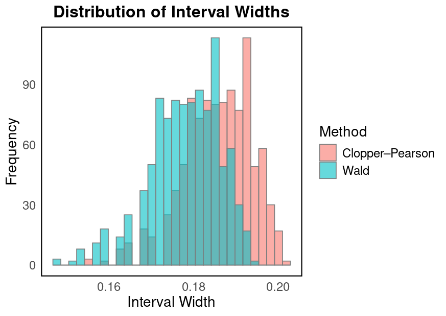
• Interval Width: Clopper–Pearson intervals are wider than Wald intervals, reflecting the trade-off between exact coverage and narrower intervals.

Visualizations

Below is a histogram comparing interval widths for Clopper–Pearson and Wald methods.

R Code for Distribution of Interval Width - Click to Expand

library(binom)      
library(ggplot2)    

set.seed(123)

p_true  <- 0.3    
n       <- 100  
N_sims  <- 1000 
alpha   <- 0.05

cp_lower  <- numeric(N_sims)  
cp_upper  <- numeric(N_sims)  
wald_lower <- numeric(N_sims) 
wald_upper <- numeric(N_sims) 
p_hat_vals <- numeric(N_sims) 

for(i in 1:N_sims) {
  k <- rbinom(1, size = n, prob = p_true)
  
  p_hat <- k / n
  p_hat_vals[i] <- p_hat
  
  cp_int <- binom.confint(x = k, n = n, conf.level = 1 - alpha, methods = "exact")
  cp_lower[i] <- cp_int$lower
  cp_upper[i] <- cp_int$upper
  
  z_val <- qnorm(1 - alpha/2)  # ~ 1.96 for alpha=0.05
  se_hat <- sqrt(p_hat * (1 - p_hat) / n)
  wald_lower[i] <- max(0, p_hat - z_val * se_hat)
  wald_upper[i] <- min(1, p_hat + z_val * se_hat)
}

# Coverage: fraction of intervals that contain p_true
cp_coverage   <- mean(p_true >= cp_lower & p_true <= cp_upper)
wald_coverage <- mean(p_true >= wald_lower & p_true <= wald_upper)

cat("Coverage (Clopper–Pearson):", cp_coverage, "\n")
cat("Coverage (Wald):           ", wald_coverage, "\n")

cp_widths   <- cp_upper   - cp_lower
wald_widths <- wald_upper - wald_lower

df_widths <- data.frame(
  Method = factor(rep(c("Clopper–Pearson", "Wald"), each = N_sims)),
  Width  = c(cp_widths, wald_widths)
)

# Histogram/frequency polygon to compare widths side-by-side
ggplot(df_widths, aes(x = Width, fill = Method)) +
  geom_histogram(alpha = 0.4, position = "identity", bins = 30) +
  labs(title = "Distribution of Interval Widths",
       x = "Interval Width", 
       y = "Frequency") +
  theme_minimal()

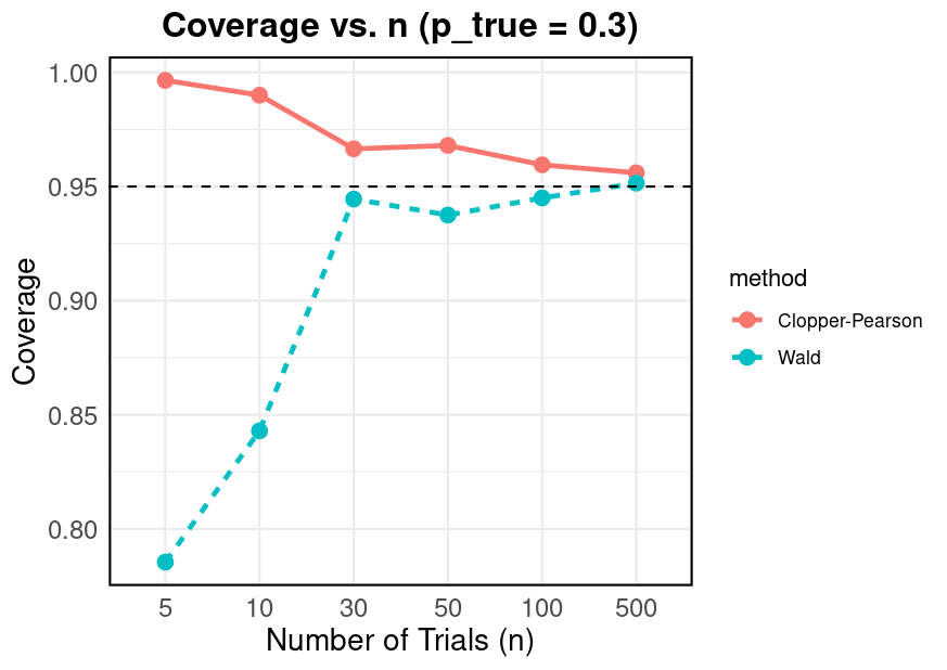
In a second simulation, I examined coverage across different sample sizes. As shown, Clopper–Pearson maintains its exact coverage (\(\ge 95\%\)) even for small sample sizes, whereas Wald intervals can dip below the nominal level.

R Code for Coverage vs. n - Click to Expand

library(binom)
library(ggplot2)

set.seed(42)

p_true    <- 0.3
n_values  <- c(5, 10, 30, 50, 100, 500)  # Example range
N_sims    <- 2000
alpha     <- 0.05

results <- data.frame(
  n = integer(),
  method = character(),
  coverage = numeric()
)

for (n in n_values) {
  cp_cover <- 0
  wald_cover <- 0
  
  for (i in seq_len(N_sims)) {
    k <- rbinom(1, size = n, prob = p_true)
    p_hat <- k / n
    
    # Clopper-Pearson
    cp_int <- binom.confint(x = k, n = n, methods = "exact", conf.level = 1 - alpha)
    cp_lower <- cp_int$lower
    cp_upper <- cp_int$upper
    cp_cover <- cp_cover + (p_true >= cp_lower & p_true <= cp_upper)
    
    # Wald
    z_val <- qnorm(1 - alpha/2)
    se_hat <- sqrt(p_hat*(1 - p_hat)/n)
    wald_lower <- max(0, p_hat - z_val*se_hat)
    wald_upper <- min(1, p_hat + z_val*se_hat)
    wald_cover <- wald_cover + (p_true >= wald_lower & p_true <= wald_upper)
  }
  
  results <- rbind(results, data.frame(n = n,
                                       method = "Clopper-Pearson",
                                       coverage = cp_cover / N_sims))
  results <- rbind(results, data.frame(n = n,
                                       method = "Wald",
                                       coverage = wald_cover / N_sims))
}

ggplot(results, aes(x = factor(n), y = coverage, color = method, group = method)) +
  geom_line(aes(linetype = method)) +
  geom_point() +
  geom_hline(yintercept = 0.95, linetype = "dashed") +
  labs(title = "Coverage vs. n (p_true = 0.3)",
       x = "Number of Trials (n)",
       y = "Coverage") +
  theme_minimal()

Summary

The Clopper–Pearson interval, rooted in the Beta distribution, demonstrates the power of exact statistical methods. While its intervals may be conservative, the guarantee of coverage makes it a reliable choice, especially for small sample sizes or extreme proportions. This exploration reinforces how the Beta distribution serves as a bridge between discrete and continuous probability frameworks, providing a deeper appreciation for its versatility in frequentist contexts.