Beta Distribution: Part 1 - Intuition and Properties

This post kicks off a series on the Beta distribution, a versatile probability distribution often used in statistics and machine learning. In this first part, I will develop an intuitive understanding of the Beta distribution and examine its fundamental properties under a Bayesian setting.

General Properties of the Beta Distribution

The Beta distribution is defined on the interval \([0,1]\). This makes it particularly convenient for modeling quantities naturally constrained between 0 and 1—such as probabilities and proportions. It is governed by two shape parameters, \(\alpha\) and \(\beta\), which determine how the distribution is skewed:

• \(\alpha\): Determines how heavily the distribution is weighted toward “success.”
• \(\beta\): Determines how heavily the distribution is weighted toward “failure.”

Probability Density Function (PDF)

The PDF of the Beta distribution is given by

\[\text{Beta}(x \mid \alpha, \beta) = \frac{x^{\alpha - 1}(1 - x)^{\beta - 1}}{B(\alpha, \beta)},\]

where \(B(\alpha, \beta)\) is the Beta function, a normalizing constant ensuring the PDF integrates to 1.

Shape of the Curve

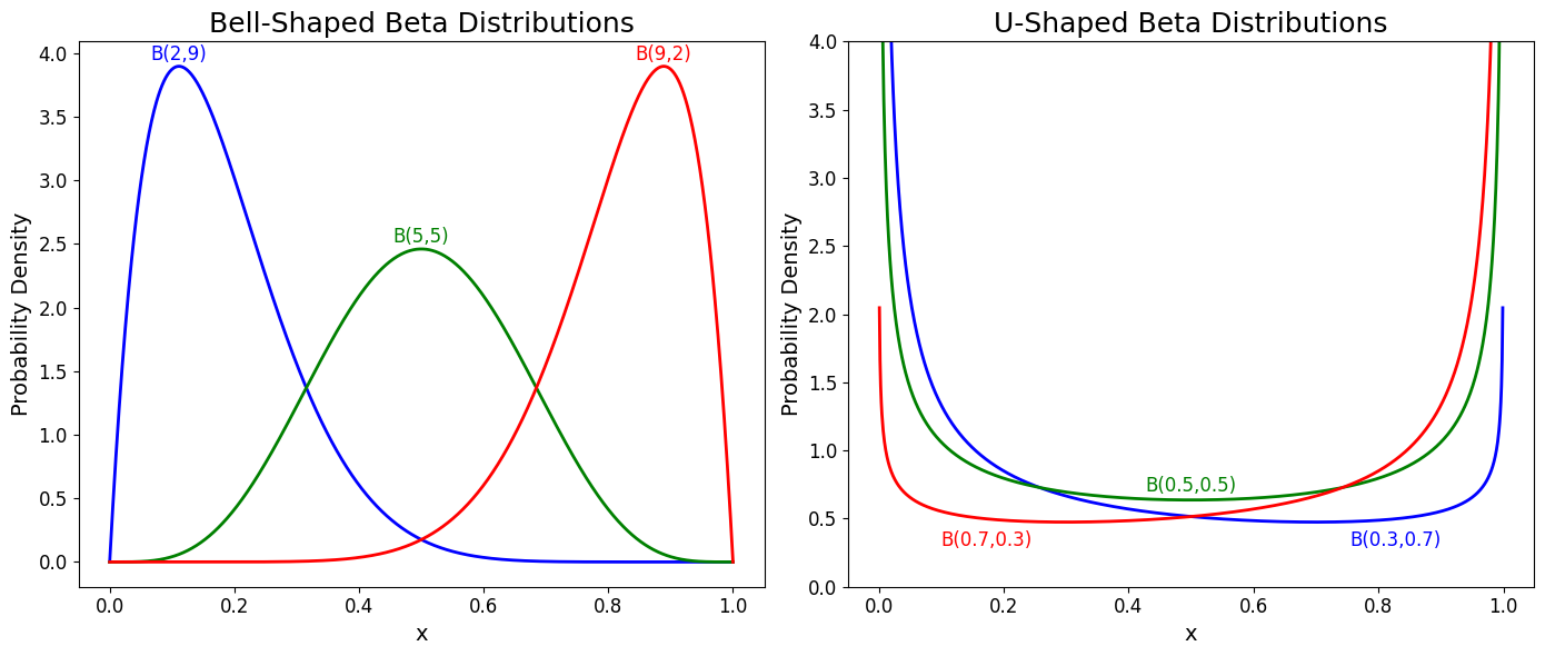
Here’s how changes in \(\alpha\) and \(\beta\) affect the shape of the distribution:

• \(\alpha = \beta = 1\): Uniform distribution on \([0,1]\).
• \(\alpha > \beta\): Skewed toward 1 (i.e., “success”).
• \(\alpha < \beta\): Skewed toward 0 (i.e., “failure”).
• \(\alpha, \beta > 1\): Bell-shaped.
• \(\alpha, \beta < 1\): U-shaped curve.

A helpful interpretation is to view the Beta distribution as a way of encoding different levels of “success” vs. “failure” weights:

\[p^{\alpha - 1} (1-p)^{\beta - 1}.\]

• No prior information: \(\alpha = \beta = 1\) yields a uniform distribution.
• Heavier weight on success (\(\alpha > \beta\)): The distribution skews toward 1.
• Heavier weight on failure (\(\alpha < \beta\)): The distribution skews toward 0.

We can also evaluate the mean (expected value) of the Beta distribution, which helps us interpret its shape and understand how \(\alpha\) and \(\beta\) influence the distribution:

\[\begin{align*} \mu = \mathbf{E}[X] &= \int_{0}^{1} x \, \frac{x^{\alpha - 1} (1 - x)^{\beta - 1}}{B(\alpha, \beta)} \, dx \\ &= \frac{\alpha}{\alpha + \beta} = \frac{1}{1 + \frac{\beta}{\alpha}}. \end{align*}\]

This shows that:

• As \(\frac{\beta}{\alpha} \to 0\), the mean \(\mu \to 1\).
• As \(\frac{\beta}{\alpha} \to \infty\), the mean \(\mu \to 0\).

Hence, when \(\alpha\) is much larger than \(\beta\), the distribution concentrates near 1, and vice versa.

Beta as a Conjugate Prior in Bayesian Inference

The Beta distribution is a conjugate prior for the Bernoulli, Binomial, and other distributions in the exponential family. This means that if we start with a Beta distribution as the prior for a parameter \(p\) (the probability of success), and then observe Binomial data (the likelihood of the data given \(p\)), the posterior distribution of \(p\) will also be a Beta distribution, but with updated parameters reflecting the new data.

Conjugacy with the Bernoulli/Binomial Likelihood

Consider a Binomial likelihood:

\[k \mid p \sim \text{Binomial}(n, p),\]

and let the prior for \(p\) be

\[p \sim \text{Beta}(\alpha, \beta).\]

After observing \(k\) successes in \(n\) trials, the posterior for \(p\) is

\[p \mid k \sim \text{Beta}(\alpha + k, \beta + n - k).\]

Because the posterior remains a Beta distribution, we say that the Beta is a conjugate prior for Bernoulli/binomial likelihoods.

Numeric Example

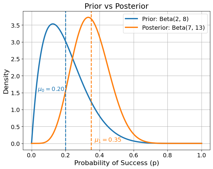
Suppose we had a prior belief that the success rate is about \(20\%\), based on historical data with 2 successes and 8 failures. Then we observe 5 successes and 5 failures. In Bayesian inference:

1. Prior: \(\text{Beta}(\alpha_0 = 2, \beta_0 = 8)\)
2. New Data: \(k=5\) successes, \(n-k=5\) failures.
3. Posterior: \(\text{Beta}(\alpha_0 + 5, \beta_0 +5) = \text{Beta}(\alpha_1 = 7, \beta_1 = 13)\)

The new posterior mean is

\[\frac{\alpha_1}{\alpha_1 + \beta_1} = \frac{7}{7+13} = \frac{7}{20} = 0.35 \quad (35\%).\]

This updated belief logically falls between the prior mean (\(20\%\)) and the naive sample estimate of \(50\%\).

Iterative (Online) Updating with the Beta Distribution

In a Bayesian framework, the Beta distribution’s conjugate properties make it ideal for iterative updating, simplifying computations when data arrives in batches. In a Bernoulli process, each new set of observations updates the Beta posterior, which seamlessly becomes the prior for subsequent data, enabling efficient step-by-step refinement.

How It Works

1. Begin with \(\text{Beta}(\alpha_0, \beta_0)\).
2. Observe \(n\) Bernoulli trials with \(k\) successes.

3. Update the prior to obtain the posterior:

   \[\mathrm{Beta}\bigl(\alpha_0 + k,\;\beta_0 + (n - k)\bigr).\]
4. The new posterior can be used as the prior for the next incoming batch of data.

Example: Iterative Updating Simulation

Below is a simulation of iterative updating for a Bernoulli process with a true success probability \(p_{\text{true}} = 0.7\). We repeatedly observe small batches of data, update our Beta prior, and watch the posterior converge to \(0.7\).

R Code for Iterative Bayesian Simulation - Click to Expand

set.seed(123)

p_true <- 0.7
n_iterations <- 5      
n_per_iter <- 10    

# Initial Beta prior parameters
alpha0 <- 2
beta0  <- 2

alpha_seq <- numeric(n_iterations + 1)
beta_seq  <- numeric(n_iterations + 1)
alpha_seq[1] <- alpha0
beta_seq[1]  <- beta0

alpha_curr <- alpha0
beta_curr  <- beta0

# Iterative Bayesian updates
for (i in 1:n_iterations) {
  # Generate Bernoulli data
  data_i <- rbinom(n_per_iter, size = 1, prob = p_true)
  
  # Update Beta parameters
  alpha_curr <- alpha_curr + sum(data_i)
  beta_curr  <- beta_curr + (n_per_iter - sum(data_i))
  
  alpha_seq[i + 1] <- alpha_curr
  beta_seq[i + 1]  <- beta_curr
}

x <- seq(0, 1, length.out = 500)
densities <- sapply(1:length(alpha_seq), function(i) dbeta(x, alpha_seq[i], beta_seq[i]))
colors <- c("black", "red", "blue", "green", "purple", "orange")

matplot(x, densities, type = "l", lwd = 2, col = colors, lty = 1,
        ylim = c(0, max(densities) * 1.05),
        xlab = "Probability of Success",
        ylab = "Density",
        main = "Iterative Bayesian Updating with a Beta Prior")

abline(v = p_true, col = "gray40", lty = 2, lwd = 2)
legend_labels <- paste0("Iteration ", 0:n_iterations, 
                        ": Beta(", alpha_seq, ", ", beta_seq, ")")
legend("topleft", legend = legend_labels, 
       col = colors, 
       lwd = 2, lty = 1, 
       cex = 0.9, bty = "n")

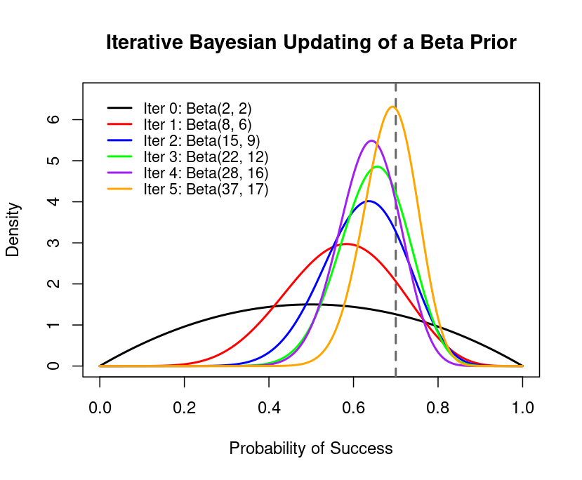
• The black curve is the initial \(\text{Beta}(\alpha_0, \beta_0)\).
• Colored curves show updated posteriors as more data arrives.
• The dashed vertical line at \(p_{\text{true}} = 0.7\) highlights how the posterior concentrates around the true value over time.

Summary

The Beta distribution models probabilities and proportions using two parameters, \(\alpha\) and \(\beta\) making it flexible to adjust. It is widely used in Bayesian inference as a conjugate prior for Bernoulli and Binomial data, allowing easy updates with new observations. This post introduced its key properties, intuition, and role in Bayesian framework.